Basketball Example • collegeballR

This example will focus on looking at SEC basketball players for 2017-2018. Data is accquired using the player_stats function found in collegeballR

library(dplyr)
library(ggplot2)
library(ggrepel)
library(data.table)
library(collegeballR)
library(rvest)
sec_urls <- "http://stats.ncaa.org/team/inst_team_list?academic_year=2018&conf_id=911&division=1&sport_code=MBB"

team_names <- read_html(sec_urls) %>% html_nodes(".css-panes a") %>% html_text()
team_names <- trimws(team_names)
teams <- team_mapping(2018,"MBB")
sec <- teams %>% filter(team_name %in% team_names) %>% mutate(
  team_id = as.numeric(team_id)
)
head(sec)

##   team_id team_name year
## 1       8   Alabama 2018
## 2      31  Arkansas 2018
## 3      37    Auburn 2018
## 4     235   Florida 2018
## 5     257   Georgia 2018
## 6     334  Kentucky 2018

sec_player_stats <- sec %>% mutate(
  team_id = as.numeric(team_id),
  player_df = purrr::map(team_id,player_stats,year=2018,sport="MBB")
)

I’ll look to incorporate a conference type function, just have to scale it out to all sports easily.

So there is an example above of using the player_stats function within purrr to get data for all SEC teams in basketball.

Cleaning Data

Let’s bring all the data into one dataframe for all teams.

sec_player_l <- sec_player_stats %>% select(player_df) %>% pull()

sec_player_df <- rbindlist(sec_player_l,fill=T) 
colnames(sec_player_df)[c(20,21)] <- c("PPG","RPG")
sec_player_df <- sec_player_df %>% inner_join(.,sec) %>% select(-G,-team_id)

Note to self, look at all sport player sites and see if Average is repeated more than once. It seems for basketball they are using Avg right after point and rebound data. It’s sort of odd, I’ll try and find a way to fix this.

sec_player_df <- sec_player_df %>% mutate(
  MP = as.numeric(gsub("\\:.*","",MP))
)

sec_player_df[,c("FGM","FGA","DRebs","Tot Reb")] <- sapply(sec_player_df[,c("FGM","FGA","DRebs","Tot Reb")],as.numeric)
head(sec_player_df)

##   Jersey             Player Yr Pos   Ht GP GS   MP FGM FGA   FG% 3FG 3FGA
## 1     05 Johnson Jr., Avery Jr   G 5-11 36  0  501  51 146 34.93  20   67
## 2     23        Petty, John Fr   G  6-5 36 28 1026 123 313 39.30  90  242
## 3     12      Ingram, Dazon So   G  6-5 35 32 1007 100 235 42.55  19   67
## 4     10     Jones, Herbert Fr   G  6-7 35 13  741  58 142 40.85   7   26
## 5     00        Hall, Donta Jr   F  6-9 34 30  806 151 208 72.60  NA   NA
## 6      4    Giddens, Daniel So   F 6-11 34 17  451  58  99 58.59  NA   NA
##    3FG%  FT FTA   FT% PTS   PPG  RPG ORebs DRebs Tot Reb AST TO STL BLK
## 1 29.85  32  40 80.00 154  4.28 1.08    12    27      39  27 19  17   1
## 2 37.19  32  45 71.11 368 10.22 2.56    14    78      92  65 74  17   9
## 3 28.36 122 177 68.93 341  9.74 5.71    33   167     200  92 79  30  12
## 4 26.92  24  48 50.00 147  4.20 3.46    29    92     121  48 56  44  22
## 5    NA  60 108 55.56 362 10.65 6.59    76   148     224  20 43  24  68
## 6    NA  28  48 58.33 144  4.24 2.53    28    58      86   8 34  14  35
##   Fouls Dbl Dbl Trpl Dbl DQ year team_name
## 1    54      NA       NA  1 2018   Alabama
## 2    36      NA       NA NA 2018   Alabama
## 3    93       2       NA  3 2018   Alabama
## 4    94      NA       NA  4 2018   Alabama
## 5    59       5       NA NA 2018   Alabama
## 6    95      NA       NA  2 2018   Alabama

But for now the data is cleaned and team names are added back. Depending on the sport you select the data will look like this, with differing stats recorded. From this you can move on to creating advanced metrics, etc.

Advanced Stats

Let’s calculate usage rate. First we need to calculate some team based stats, before calculating USG rate.

sec_p_df <- sec_player_df %>% group_by(team_name) %>% mutate(
  team_minutes = sum(MP,na.rm=T),
  team_FGA = sum(FGA,na.rm=T),
  team_FTA = sum(FTA,na.rm=T),
  team_TO =  sum(TO,na.rm=T)
) %>% ungroup() %>% as.data.frame()
sec_p_df[is.na(sec_p_df)] <- 0
sec_p_df <- sec_p_df %>% mutate(
  usg_rate = 100 * ((FGA + 0.475 * FTA + TO) * (team_minutes/5)) / (MP * (team_FGA + 0.475 * team_FTA + team_TO))
  )

Plotting

ind_df <- sec_p_df %>% filter(MP>100)
labels <- ind_df %>% filter(usg_rate>25 & MP > 750)
ggplot() +
  geom_point(data = ind_df, aes(y = MP, x = usg_rate, color = team_name)) + theme_bw(base_size=16) +
  geom_text_repel(data = labels, aes(x = usg_rate, y = MP, label = Player)) +
  facet_wrap(~team_name) + 
  labs(x = "Usage Rate", y = "Minutes", caption = "@msubbaiah1",
       title = "SEC Basketball Usage Rate by team",
       subtitle = "2017 - 2018 season") + 
  theme(legend.position = "none")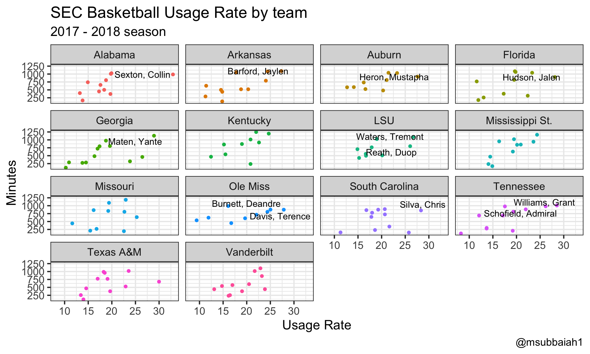

There is the basics of getting player data from collegeballR!